Logistic regression is actually a classification model. In linear regression, we construct a hyperplane that passes through all data points as closely as possible. Logistic regression, on the other hand, does the opposite — it separates samples into two groups as much as possible, maximizing the probability that each sample belongs to its assigned class. Of course, this class assignment is prior information, so logistic regression is a type of supervised learning. This article implements binary logistic regression using both gradient descent and Newton's method.
A Simple Binary Classification Model
Consider the ideal case: if we could find a function that takes a sample as input and outputs 1 when the sample belongs to class 1, or 0 when it belongs to class 2. The sign function fits our needs — for any , its output is either 0 or 1.
This sounds ideal, but the sign function is not practical to use. One reason is that it is discontinuous over its domain. If we want to compute derivatives or perform other operations on it, it becomes extremely difficult. Therefore, it would be great to have a function that resembles the sign function, is continuous over its domain, and is also higher-order differentiable. Fortunately, we found the logistic function, shown as the purple curve in the figure.
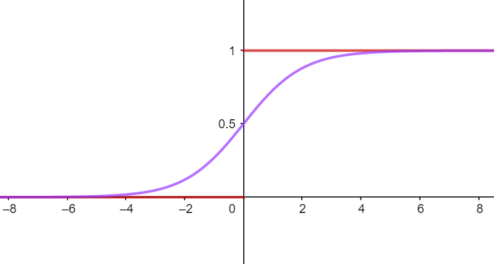
The logistic function maps the sample to the range . It is monotonically differentiable and has excellent mathematical properties. Its mathematical form is:
The next step is straightforward: given the different features in the samples, we want to find appropriate to multiply with them, sum the results, and feed them into the function, then classify according to the following rule:
Thus, the problem reduces to finding an appropriate set of such that all samples are classified into their correct categories as accurately as possible. Consider the maximum likelihood function:
where are respectively:
To ensure each sample is classified as correctly as possible, we need to maximize the likelihood function.
Computing the product is difficult, so we generally use the log maximum likelihood estimation, which is essentially equivalent for finding the maximum. By convention, we add a negative sign, turning it into a problem of minimizing the negative log-likelihood function. In fact, the negative log-likelihood function is also convex, so we can still use the gradient descent method learned in linear regression.
where is the learning rate and is the gradient of the negative log-likelihood function.
In addition, it is worth learning another method: Newton's method.
Let me briefly explain the principle here.
Consider the Taylor expansion of a continuous, higher-order differentiable function around a neighborhood of , and take the first two terms:
Setting , we get:
So, if has a solution, we can always obtain it through iteration.
And we know that is convex, so the minimum is located at the point where the derivative is zero. We can iterate on the derivative of the function, achieving the same result as with the original function.
Gradient Descent Method
Formula Preparation
For convenience, let us first derive the derivative of the function
And the cost function
Taking the derivative of the cost function gives:
And vectorizing for efficient computation:
In summary, we obtain the iteration formula:
As long as we implement the above process in code, it is easy to get the desired program.
Python Implementation
Import libraries:
import numpy as np
import pandas as pd
import time
import data_in # 导入数据
import matplotlib.pyplot as plt
Data loading and preprocessing:
def data_np_lr(): # 数据导入
	return np.array(pd.read_table('./data/LR_data.txt'))
def normalization(data): # 归一化, 并对X添加一列常数项
    ones = np.ones((data.shape[0], 1))
    data = (data - np.min(data, axis=0)) / (np.max(data, axis=0) - np.min(data, axis=0))
    return  np.append(ones, data, axis=1)
Gradient descent implementation:
# 定义Sigmoid函数
def sigmoid(z):
    return 1.0 / (1.0 + np.exp(-z))
# 定义成本函数
def cost(X, theta, y):
    m, n = X.shape
    h = sigmoid((np.dot(X,theta)))
    cost = (-1.0/m) * np.sum(y.T * np.log(h)
                             + (1- y).T * np.log( 1 - h))
    return cost
# 梯度迭代下降
def LR_gradient(X, y, alpha=0.01, tol=1e-4, max_iter=100000):
    process = max_iter / 100  # 显示进度
    # matrix 更为方便
    X = np.mat(X)
    y = np.mat(y)
    m, n = X.shape
    theta = np.ones((n, 1))
    loss = 1
    iter = 0

    while (iter < max_iter):
        loss = cost(X, theta, y)
        # 梯度的下降法
        h = sigmoid(np.dot(X, theta))  # 预测值
        error = h - y  # 误差项
        grad = (1.0 / m) * np.dot(X.T, error)  # 梯度
        theta = theta - alpha * grad

        if (iter % process == 0):
            print("|", end="")
        if np.all(np.absolute(grad) <= tol):
            break
        iter += 1
    print("\n迭代:", iter, "次", "  最大迭代次数: ", max_iter, "损失: ", loss)
    return theta
Prediction results:
def predict(X, theta, y):
    m, n = X.shape
    pre = np.zeros((m,1))

    for i in range(m):
        map = sigmoid(np.dot(X[i,:],theta))
        if map > 0.5:
            pre[i] = 1

    count = 0
    for i in range(m):
        if (pre[i] == y[i]):
            count +=1
    return count / m
Result visualization:
def paint_result(X, y, w):
    fig = plt.figure()
    ax = fig.add_subplot(111)
    for i in range(X.shape[0]):
        if y[i] == 1:
            ax.scatter(X[i][1], X[i][2],color="red")
        else :
            ax.scatter(X[i][1], X[i][2], color="green")
    x = np.arange(min(X[:,1]),max(X[:,1]),0.001)
    y = (-w[0] - w[1] * x.T)/w[2]
    ax.plot(x, y.getA1())
    plt.show()
Main function:
if __name__ == '__min__':
    file_read = data_in.data_np_lr() # 小规模训练集
    rows, columns = file_read.shape
    beta = 0.8 # 训练集占比
    # 训练集
    X_tr = normalization(file_read[:int(rows*beta), :columns - 1])
    y_tr = file_read[:int(rows*beta), -1:]

    # 测试集
    X_test = normalization(file_read[int(rows*beta):, :columns - 1])
    y_test = file_read[int(rows*beta):,-1:]

    print("Logistic Regression 梯度下降算法")
    time_start = time.time()
    theta_1 = LR_gradient(X_tr, y_tr,alpha=0.05, tol=1e-4,max_iter=1e6)
    time_end = time.time()
    print("测试集预测准确率: ",predict(X_test,theta_1,y_test),end="//")
    print('time cost', time_end - time_start, 's')
    # 绘制结果
    paint_result(X_tr, y_tr, theta_1)
    paint_result(X_test, y_test, theta_1)
Viewing the Results
First, let's look at the function output:
Logistic Regression 梯度下降算法
迭代: 594006 次 最大迭代次数: 1000000.0 损失: 0.09410151721717233
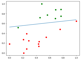
测试集预测准确率: 0.95//time cost 53.365071296691895 sVisualizing the data, let's look at the training set iteration results:
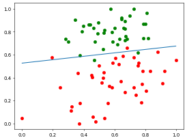
Using the test set to evaluate the training results:
 The results are impressive!
Newton's Method
Newton's method is very similar to gradient descent; the only difference is that the iteration process has an additional step — computing the second-order derivative.
Code Implementation:
Similar to the code above, just add:
def newtons_method_gradient(X, theta ,y): # 求解一阶偏导
    m, n= X.shape
    return (1.0/m) * np.dot(X.T, sigmoid( np.dot(X, theta)) - y)

def newtons_method_hessian(X, theta ,y): # 负最大对数似然函数的二阶Hessian矩阵
    p = sigmoid( np.dot(X, theta))
    q = p.getA1()
    '''
    p 必须使用getA1()方法转化为一维的数组.
    在numpy中, array([12, 23, 34]) 和 array([[12, 23, 34]])并不完全相同
    而在此处, 可能由于版本原因, 很多网上很多教程使用np.diag(array([[]]))是
    可以得到正常的对角矩阵的, 而我的环境已经不支持这样做了, 只会一维矩阵的形式返回
    结果
    所以, 必须使用getA1()方法, 将p强制转换为数组, 这样np.diag()方法才能将数组正常
    地转化为对角矩阵, 而不是以一维数组的方式返回
    '''
    return (1.0/m)*X.T.dot(np.diag(q * (1-q)).dot(X))

def LR_newton(X, y, tol = 1e-6, max_iter = 10000):
    process= max_iter / 100
    X = np.mat(X)
    y = np.mat(y)
    m, n = X.shape
    theta = np.zeros((n,1))
    loss = 1
    iter = 0
    while( iter < max_iter):
        loss = cost(X,theta, y)
        # 牛顿迭代法
        grad = newtons_method_gradient(X, theta, y)
        hessian = newtons_method_hessian(X, theta, y)
        theta = theta - np.linalg.inv(hessian) * grad
        if iter % process == 0:
            print("|",end="")
        if np.all(np.absolute(grad) <= tol):
            break
        iter += 1

    print("\n迭代:",iter,"次",",最大迭代次数: ", max_iter, "损失: ",loss)
    return theta
Simply call the function:
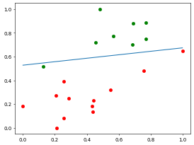
theta_1 = LR_newton(X_tr, y_tr, tol=1e-5,max_iter=1e5)Output:
Logistic Regression 牛顿迭代法
迭代: 7 次 ,最大迭代次数:  10000.0 损失:  0.09400816347426497
测试集预测准确率:  0.95//time cost 0.001995563507080078 s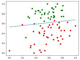
As we can see, Newton's method achieves a very small loss function value with fewer iterations, and under suitable conditions, it can even produce faster results than gradient descent.
Moreover, Newton's method does not require manually setting the step size, eliminating many of the hassles involved in hyperparameter tuning.
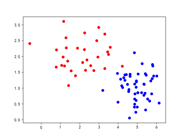
Tip: How to Create Your Own Sample Data
When doing assignments, you might find that the dataset provided by the course is very large and the training results are not great. As a beginner, this can be very confusing — you might wonder if you made a mistake, or sometimes you want to verify whether your method is correct, but training takes a long time. Therefore, we can construct a smaller, controllable data sample as our training set.
# 生成80个数据
    for i in range(50):
        # 归于蓝方
        one = random.gauss(5, 0.5) # 均值, 标准差
        two = random.gauss(1,0.5)
        x_1.append(one)
        x_2.append(two)

    for i in range(30):
        # 归于红方
        one = random.gauss(2,1)
        two = random.gauss(2,0.5)
        y_1.append(one)
        y_2.append(two)
    plt.scatter(x_1, x_2, color="blue")
    plt.scatter(y_1, y_2,color="red")
    plt.show()
The code here is written for plotting convenience. In practice, you can directly generate a numpy matrix. This way, as long as we specify some distribution parameters, we can create an elegant dataset. In fact, the cover image dataset was generated using this very code!
Login to Comment
You need to log in to leave a comment.
Login